Howdy Neighbor! Proximity Analysis in R

The sf library makes it relatively straightforward to create distance based buffers with the st_buffer operation where the two key imports are the name of the sf object with the features around which to buffer and the buffer distance in the units of the CRS of the sf object. For the CA Albers CRS the units are meters.  In the code below we define a buffer distance of 2000 meters, or 2km. This will define areas that are 2KM around each point. We may wish to do this if our assumption is that people use the closest hospital if it is within 2KM. We know that to be an oversimplification!

# Identify buffer distance in units of the CRS, here meters

bufdist <- 2000  # or 2km

# Implement the buffer operation on the points

# which outputs polygons for each point

pts_buf <- st_buffer(my_pts, dist=bufdist)

# Plot results

plot(my_poly$geometry)

plot(pts_buf$geometry, add=T)

plot(my_pts$geometry, col="red", add=T)

 

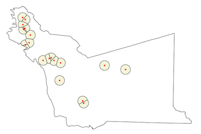
Now those buffers are all the same size regardless of the number of hospital beds. So let’s vary the size of the buffers based on the number of beds. The way we do this is as follows. 

• First we use the classInt::classIntervals function to create a set of break points based on binning the points into 5 quantiles based on the number of beds. 
• We then use those class breaks to create a bed_weight variable that ranges from 1-5 for each quantile.
• We set the initial buffer size to 1000 meters and then multiply it by the bed_weight to get a buffer distance that ranges from 1 to 5 KM.

# Take a look at the range of values for number of beds

summary(as.numeric(my_pts$TOTAL_NUMBER_BEDS))

# make the number of beds an integer variable

my_pts$TOTAL_NUMBER_BEDS <- as.numeric(my_pts$TOTAL_NUMBER_BEDS)

# Now lets use the classInt package to classify the number of beds into weights

# depending on what quantile they fall into

my_cats <- classIntervals(my_pts$TOTAL_NUMBER_BEDS, n=5, style="quantile")

my_cats

names(my_cats)

# Make a weights vector that we can add back to the dataframe

my_weights <- cut(my_pts$TOTAL_NUMBER_BEDS, breaks = my_cats$brks, labels=as.numeric(1:5))

length(my_weights)

nrow(my_pts)

my_pts$bed_weights <- cut(my_pts$TOTAL_NUMBER_BEDS, breaks = my_cats$brks, labels=F)

#Check the shape of the bed_weights var

summary(my_pts$bed_weights)

# if any weights are NA set them to one

my_pts$bed_weights[is.na(my_pts$bed_weights)] <- 1

# Now create a buffer that multiplies our base distance times the weight

bufdist = 1000

pts_bufw <- st_buffer(my_pts, (bufdist*my_pts$bed_weights))

#finally, map the output

plot(my_poly$geometry)

plot(pts_bufw$geometry, add=T)

plot(my_pts$geometry, col="red", add=T)

 

Our variable distance polygons take into account the ability of a hospital with a lot of beds to service a larger area.

VORONOI DIAGRAM

Our buffer polygons do not account for all of the area around a hospital, e.g., if an area isn’t in the buffer it is not assigned to a hospital. But we know that everyone may need to go to a hospital at some point. So let’s consider how a Voronoi diagram can be used to model proximity.

In the code below, after that from Dan Houghton on github, we partition all of Alameda County so that each area within it is assigned to the nearest hospital.

voronoi <- 

  my_pts %>% 

  st_geometry() %>%

  st_union() %>%

  st_voronoi() %>%

  st_collection_extract()

# Put output back in their original order

# so can easily rejoin with source attributes

voronoi <-

  voronoi[unlist(st_intersects(my_pts,voronoi))]

# Plot the point voronoi polygons

plot(voronoi)

# clip the voronoi polys to the boundary

voronoi2 <- st_intersection(my_poly$geometry, voronoi)

# plot the clipped voronoi polygons

plot(voronoi2)

plot(my_pts$geometry, add=T, col="red", pch=20)

# Make the voronoi polygon data an sf object

# that has the voronoi geometry but the input attributes

voronoi_sf = st_sf(my_pts, geometry = voronoi2)    # sf object

st_set_crs(voronoi_sf, my_crs_code)

st_crs(voronoi_sf)

# Plot it to check

plot(voronoi_sf$geometry)

plot(my_pts$geometry, add=T, col="red", pch=20)

 

COMBINING BUFFERS AND VORONOI POLYGONS

 We can combine these two approaches as a way of implementing the assumption that an area will be served by the closest hospital, but only within a specific distance.

 Here we implement this combining Voronoi polygons clipped to fixed distance buffers, again following code by Dan Houghton:

st_buffer_without_overlap <- function(centroids, dist) {

  # Voronoi tesselation

  voronoi <- 

    centroids %>% 

    st_geometry() %>%

    st_union() %>%

    st_voronoi() %>%

    st_collection_extract()

  # Put them back in their original order

  voronoi <-

    voronoi[unlist(st_intersects(centroids,voronoi))]

  # Keep the attributes

  result <- centroids

  # Intersect voronoi zones with buffer zones

  st_geometry(result) <-

    mapply(function(x,y) st_intersection(x,y),

           st_buffer(st_geometry(centroids),dist), 

           voronoi,

           SIMPLIFY=FALSE) %>%

    st_sfc(crs=st_crs(centroids))

  result

}

buffer_distance_meters <- 2000 # 2000 meters or 2 km

pts_buffered <- st_buffer_without_overlap(my_pts, buffer_distance_meters)

# Plot buffer points

plot(my_poly$geometry)

plot(pts_buffered$geometry, add=T)

# Clip buffer points

pts_buffered_clipped <- st_intersection(my_poly, pts_buffered)

# plot clipped points

plot(my_poly$geometry) 

plot(pts_buffered_clipped, col="beige", add=T)

plot(my_pts$geometry, pch=20, col="red", add=T)

Here we implement same approach with with variable width buffers

st_buffer_without_overlap_weighted <- function(centroids, dist, weight_var) {

  # Voronoi tesselation

  voronoi <- 

    centroids %>% 

    st_geometry() %>%

    st_union() %>%

    st_voronoi() %>%

    st_collection_extract()

  # Put them back in their original order

  voronoi <-

    voronoi[unlist(st_intersects(centroids,voronoi))]

  # Keep the attributes

  result <- centroids

  # Intersect voronoi zones with buffer zones

  st_geometry(result) <-

    mapply(function(x,y) st_intersection(x,y),

           st_buffer(st_geometry(centroids), (dist*centroids[[weight_var]])), 

           voronoi,

           SIMPLIFY=FALSE) %>%

    st_sfc(crs=st_crs(centroids))

  result

}

#

buffer_distance_meters <- 1000 # 20000 meters or 20 km

pts_buffered2 <- st_buffer_without_overlap_weighted(my_pts, buffer_distance_meters, 'bed_weights')

# Plot buffer points

plot(my_pts$geometry)

plot(pts_buffered2$geometry, add=T)

# clip 

pts_buffered_clipped2 <- st_intersection(my_poly, pts_buffered2)

# plot clipped points

plot(my_poly$geometry) 

plot(pts_buffered_clipped2, col="beige", add=T)

plot(my_pts$geometry, pch=20, col="red", add=T)

 

WEIGHTED VORONOI DIAGRAM

For our final example, we are going to implement code to create a weighted Voronoi diagram as a way to partition the study area but giving more weight to hospitals with a larger bed capacity. This code is borrowed from two Stack Overflow posts, one by Dr. William Huber that describes Thiessen polygons in detail, and one by Simone Bianchi who provide code for how to implement their creation in R. I recommend that you read both of these posts. I provide the code here so that you can see how to implement it with sf objects in R using data that is available online. In this example, we use the bed weights to multiplicatively vary the size of the Voronoi polygons around each point. Following Bianchi, we implement a raster implementation due to the computation complexity of generating a vector weighted Voronoi partition.  This assumes some knowledge of raster data structures and methods in R.

################

# weighted voronoi

################

rez= 1000 # this number is the cell size and depends on the size of the study area

maxlen=603 # WHERE DID 603 come from? It should be the distance / rez

my_id_var <- 'OSHPD_ID'

my_weight_var <- 'bed_weights'

r <- raster(xmn=sf::st_bbox(my_poly)[['xmin']], 

            xmx=(sf::st_bbox(my_poly)[['xmin']] + (maxlen*rez)), 

            ymn=sf::st_bbox(my_poly)[['ymin']], 

            ymx=(sf::st_bbox(my_poly)[['ymin']] + (maxlen*rez)), 

            crs = sf::st_crs(my_poly)$proj4string, resolution=rez)

pts_dt <- data.table(

  ptID = paste0('x',my_pts[[my_id_var]]),  # ID MUST BE A STR and UNIQUE

  x = st_coordinates(my_pts)[,1] ,

  y = st_coordinates(my_pts)[,2],

  size=my_pts[[my_weight_var]]

)

head(pts_dt)

# create an empty datatable with the length equal to the raster size

dt <- data.table(V1=seq(1, length.out = (maxlen*rez)^2*(1/rez)^2))

# calculate distance grid for each tree, apply weight and store the data

for (i in pts_dt[, unique(ptID)]){

  #print(i)

  # 1) standard Euclidean distance between each cell and each point

  d <- distanceFromPoints(r, pts_dt[ptID==i,.(x,y)])

  # 2) apply your own custom weight

  # modify distance values by point weight (should set weight default to 1)

  d <- ((d@data@values)^2)/pts_dt[ptID==i,size]

  # 3) store the results with the correct name

  dt <- cbind(dt,d)

  #print(i)

  setnames(dt, "d", i)

}

# carry out comparison

# find the column with the lowest value (+1 to account to column V1 at the beginning)

# ie. find the smallest distance between a cell and a point

dt2<-dt

dt[,minval:=which.min(.SD)+1, by=V1, .SDcols=2:length(names(dt))]

# find the name of that column, that is the id of the point

dt[,minlab:=names(dt)[minval]]

# create resulting raster

out <- raster(xmn=sf::st_bbox(my_poly)[['xmin']], 

              xmx=(sf::st_bbox(my_poly)[['xmin']] + (maxlen*rez)), 

              ymn=sf::st_bbox(my_poly)[['ymin']], 

              ymx=(sf::st_bbox(my_poly)[['ymin']] + (maxlen*rez)), 

              crs = sf::st_crs(my_poly)$proj4string, resolution=rez,

              vals=dt[,as.factor(minlab)]

)

plot(out)

out_masked <- mask(out, my_poly)

plot(out_masked)

plot(my_poly, add=T)

# Transform into polygons

# Note outpt is class sp

outpoly <- rasterToPolygons(out_masked, dissolve=T)

outpoly_sf <-st_as_sf(outpoly)

# add the point ids to the polys

x <- dt[,as.factor(minlab)]

outpoly_sf$nearpt_id <- levels(x)[outpoly_sf$layer]

# Plot results with starting points

plot(outpoly_sf$geometry, col="beige");

plot(my_pts$geometry, col="red",add=T)

 

Voronoi and Weighted Voronoi polygons partition space into neighborhoods with similar estimated characteristics, hospital service areas in this example. As such, Voronoi diagrams are a method of spatial interpolation. These polygons can also serve as inputs to adjacency based methods of proximity analysis such as spatial autocorrelation, which considers patterns and trends in the data. Spatial analysis provides many ways to consider neighborliness.

CONCLUDING THOUGHTS

That’s a lot of proximity analysis code to chew on! I hope that there is some useful code in this post, whatever type of neighborhood you are trying to model.  I also hope you can see from this post just how powerful R is as a computing environment for spatial analysis. The R sf and raster packages and related libraries provide a fantastic complement to desktop GIS software like ArcGIS and QGIS.  If you want to learn more, register for the D-Lab’s R Geospatial Data Fundamentals workshop, one iteration of which will be held in March 2021. I also strongly (and often) recommend the great online book Geocomputation with R by Robin Lovelace, Jakub Nowosad, and Jannes Muenchow for those interested in geospatial data and analysis in R.