Mapping Time-Series Satellite Images with Google Earth Engine API

Mapping Time-Series Satellite Images with Google Earth Engine API

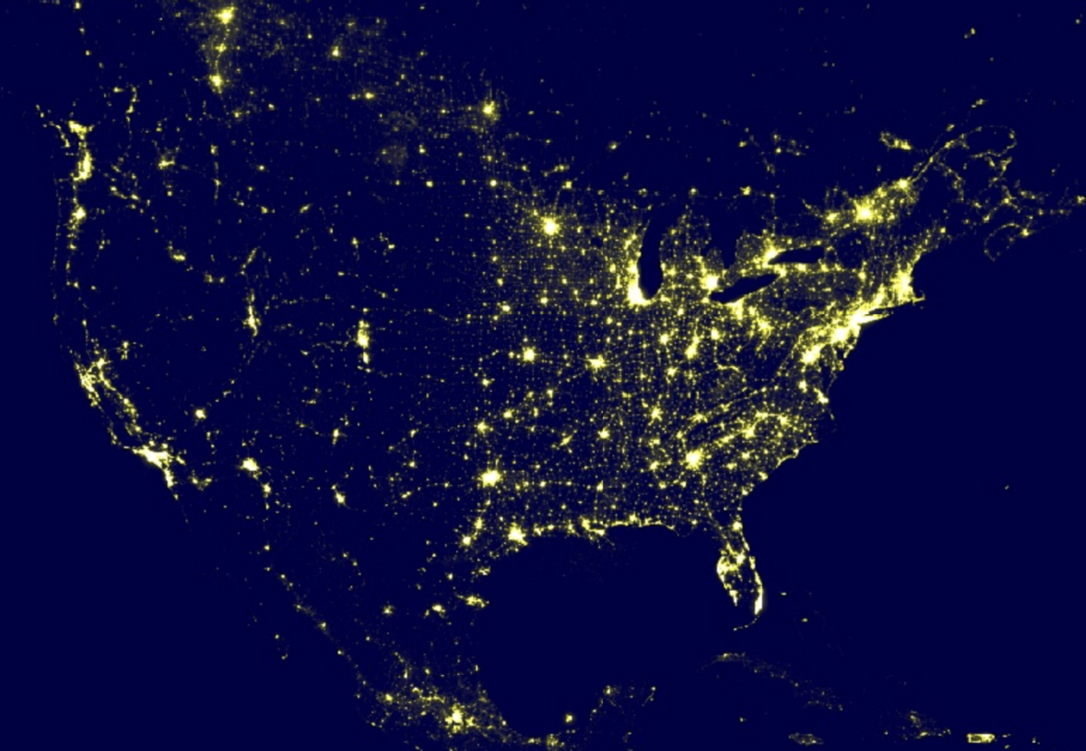
Remote sensing imagery such as satellite imagery has the potential to reveal land use patterns and human activities at a planetary scale. For example, nighttime light intensity extracted from satellite images can identify areas with high concentrations of human settlements and activities, especially in locations where traditional data are scarce. Google Earth Engine (GEE) is a general purpose tool capable of extracting time-series remote sensing data from the GEE Data Catalog.In this blog post, I walk through the process of using the GEE to obtain remote sensing data, filter it by time and geographic region, and finally visualize the data on static and interactive maps. 

Full demonstration code and examples can be found at this Google Colab notebook.

API Setup

There are two ways to access GEE: either through the Earth Engine Code Editor or via an API in Python or Javascript. The API allows for flexibility to integrate Earth Engine (EE) with the project workflow. Before using the API, you will need to sign up for Earth Engine Access, which grants access to the Code Editor and API. You will need to proceed through several steps to authenticate and initialize the EE Python client library, which are detailed both in my Colab notebook and the GEE documentation.

Explore the Earth Engine Data Catalog

The Earth Engine Data Catalog has a variety of public raster datasets, including daytime and nighttime satellite imagery, which we can import directly to our projects by referencing an  "Earth Engine Snippet". An “Earth Engine Snippet” is a piece of unique identifier for users to search and access geospatial data such as image collection and feature collection, hosted on the GEE platform. The two datasets I use for this project are:

1. CCNL: Consistent And Corrected Nighttime Light Dataset from DMSP-OLS (1992-2013)

2. VIIRS Stray Light Corrected Nighttime Day/Night Band Composites Version 1

The Earth Engine Snippet for the CCNL dataset, for example, is “BNU/FGS/CCNL/v1” as is shown in the following screenshot. 

CCNL DMSP/OLS Dataset

CCNL stands for consistent and corrected nighttime lights, which is a reprocessed version of the Defense Meteorological Program (DMSP) Operational Line-Scan System (OLS) Version 4 data. It is an annual time-series dataset of the global nighttime light intensity from 1992 to 2013. 

We can use ee.ImageCollection to import the CCNL dataset ( ‘b1’ is the band with corrected nighttime light intensity values). I select data from the whole date range between January 1st, 1992 and January 1st, 2014:

VIIRS Dataset

An updated version from the DMSP/OLS dataset whose coverage ends by the end of 2013, is the Visible Infrared Imaging Radiometer Suite (VIIRS), a monthly average radiance composite image collection from 2014 to 2022. This dataset has a higher resolution that captures more variations in nighttime light intensity than the earlier DMSP/OLS dataset. 

We import the VIIRS dataset from the ‘avg_rad’ band for the whole date range. 

Import Custom Features

In order to conduct more focused analysis, I upload two custom feature tables that include California county and state boundaries. Once the shapefiles are uploaded, GEE generates a EE snippet of the feature or feature collection which we can directly import into our project. 

Get Time-Series Data for a Location

Let’s compare the CCNL and VIIRS datasets in terms of the average nighttime light intensity values and variations across time around our point of interest. First, we restrict the time-series data from both datasets to UC Berkeley’s campus (i.e., [-122.3790, 37.6213]). We can use .getRegion() to calculate the average nighttime light intensity across years:

The following scatter plot visualizes the temporal variations of nighttime light intensity from 1992 to 2022 around UC Berkeley. Note that the green dots are denser than the purple ones because VIIRS updates more frequently than DMSP/OLS. Overall, the DMSP/OLS nighttime light intensity values exhibit a higher range than the VIIRS values. 

Static Image

Instead of a single location, we can extract the average values of each pixel from an entire region. In this example, we filter the data by Alameda County, and visualize them in a customized color palette. 

The images below depict 1) the mean DMSP/OLS values of Alameda County throughout the years between 1992 and 2013 (left) and 2) the mean VIIRS values between 2014 and 2022 (right). Comparing the two thumbnails using DMSP/OLS and VIIRS, we see the latter has a higher resolution and less overcast. 

We can save the two thumbnails as GeoTIFFs into Google Drive or download them from a generated link. 

Interactive Map

The final step is to map the global nighttime light data onto an interactive map. In this map, we overlap the mean values of the whole nighttime light datasets on top of the global OpenStreetMap. We can play around with it in the demonstration notebook. Toggle between DMSP and VIIRS layers by clicking checkboxes on the top right. We will observe a lot of interesting patterns of urban agglomeration, network and clusters of cities, etc.  

All in all, I find GEE is a really useful tool to facilitate planetary-scale raster data processing, which could be helpful for land use and environmental planning, as well as serving as an interactive mapping tool to explore the Earth’s surface. There are plenty of resources available online discussing the various capabilities of using GEE. Feel free to shoot me an email if you would like to chat about ideas working with this tool! 

References

1. Li, Meiqing. (2018). Estimating County-level Urban Intensity using Google Earth Engine: A case of California, American Association of Geographers Annual Meeting.

2. Earth Engine Python API Colab Setup: https://colab.research.google.com/github/google/earthengine-api/blob/master/python/examples/ipynb/ee-api-colab-setup.ipynb

3. An Intro to the Earth Engine Python API: https://colab.research.google.com/github/google/earthengine-community/blob/master/tutorials/intro-to-python-api/index.ipynb