Understanding Rock Climbing using Python & SQL

Understanding Rock Climbing using Python & SQL

The Rise of Climbing

As an avid rock climber, I’ve been curious about how climbing became so popular in such a brief time, and what these climbers look like. Unlike other well established sports such as tennis, football, or basketball, climbing has only recently gained attention on the public stage, and little data is available about this burgeoning sport.For context, back in the day, climbing was a serious commitment! You had to find a buddy to learn how to use climbing equipment, buy your own equipment, seek out climbing locations, and invest in long trips to the mountains. With the massive growth of indoor climbing gyms, all of these barriers to entry have faded away and, as a result, the climbing gym industry grew by 4.8% on average over the past seven years (https://my.ibisworld.com/us/en/industry-specialized/od4377/industry-at-a-glance). 

Whilst data exists for professional climbers from competitions, there is less data about the average joe-schmoe climbers like myself. Hence, I went on a journey to discover key insights about these climbers using both my domain knowledge in the sport and my data science skills. Nothing gets more Bay Area than this!

The Sport of Climbing

Before diving into the data, I will define a few key terms you will need to understand climbing jargon.

1. Bouldering - Climbing a smaller rock a.k.a. "boulder" without ropes. Typically short and difficult, requiring power.
2. Route - Climbing a longer mountain-side "route" using a rope. Typically long, requiring endurance.
3. Send or Ascent - Successfully climbing to the top of a route or boulder.
4. Grade - The difficulty of a climb. Grading a route or boulder can be subjective. On top of that, there are separate grading systems for routes and boulders. And on top of THAT, there are different US and European grading systems! See https://rockandice.com/how-to-climb/climbing-grades-explained/ for more details on this complex system!

The Data Hunt

In an exploratory data analysis, asking the right questions and searching for datasets that can answer those questions is an iterative process. You may start with a set of questions, only to later realize that they can’t be answered given the data available. On the other hand, you may find datasets that have information to answer questions you didn't initially consider.

I started with questions such as:

1. How has climbing participation grown over the past several decades?
2. What is the maximum V-grade for the average climber?
3. What is the average height/weight of climbers? 

With these preliminary topics in mind, I went on the hunt for datasets that might answer these questions, and found two promising candidates:

1. A reddit climber survey (https://www.reddit.com/r/climbharder/comments/6693ua/climbharder_survey_results/)
2. A kaggle database of users from the largest rock climbing logbook 8a.nu (https://www.kaggle.com/dcohen21/8anu-climbing-logbook)

Dataset Tradeoffs

The reddit survey data has around 600 records with 34 features including sex, height, weight, age, years climbing, maximum climbing grade acheived, maximum consective pullups, while the kaggle 8a.nu dataset has over 60,000 user records including sex, height, weight, age, years climbing, occupation, and every route they logged on the website.

While the reddit data was much richer, these extra features didn’t answer some of my main questions. Additionally, extrapolating a community of millions of people from a sample size of 600 voluntary responses to a survey may not accurately represent average climbers. Instead, I went with the kaggle 8a.nu dataset for my analysis since it had 100-fold records, and contained the features I needed.

Only later would I discover that this dataset would require extra tools outside of my familiarity to pry open and analyze.

Python

For many readers of this blog, you may be familiar with Python, which consistently tops the list as the most widely used programming language in data science applications (https://www.datacamp.com/blog/top-programming-languages-for-data-scientists-in-2022). One of the most common data structures used to load in, wrangle, and analyze data is in the dataframe. 

Dataframes are great for their simplicity, functioning like any good old excel spreadsheet with rows as samples and columns as features. The raw data imported into Python for dataframes is typically a csv (comma separated value) file which is easily imported into Python using the pandas library such as:

import pandas as pddataframe = pd.read_csv("path_to_csv_directory/my_file.csv")

Unfortunately, the kaggle 8a.nu dataset is not in a csv format, but in a SQL (Structured Query Language) database, oh my! So, are we doomed and better off looking for a simpler dataset to analyze? Never!

An intermission: As we dive into the world of SQL…

SQL & Relational Databases

Why use a SQL database instead of a csv file? 

As a case study, imagine you are in charge of dealing with product transactional data on Amazon. You are asked to create a database that tracks every time a customer purchases some product. We need tons of information on the user, product, and transaction information. If we use a csv, each row would be a transaction and would include dozens, or hundreds of rows that contain information about both the user and the product. 

Let’s say a single user buys the same product multiple times. Well we need to track all the information for each purchase!

Just to imagine this at scale, say we have 40 features for each user, 50 features for each product, and 10 features for each transaction. For every purchase, we would add 100 new values to our csv table. Amazon ships about 1.6 million orders everyday (https://querysprout.com/how-many-orders-does-amazon-get-every-second-minute-hour). So how does this scale our csv database?

1,600,000 x 100 = 100,600,000 

Every day we would add over one hundred million values to our csv database! Can we do better? 

This is where relational databases come into the picture! Instead of replicating product and user data for every purchase, we instead just refer to a product and user table that stores this information for when we actually need it. In this paradigm, we now have three tabular tables, a user table, a product table, and a transaction table. Now when we need to update our relational database, we only need to update the 10 transaction features, and the references to our user and product table adding only 12 new values! So how much fewer records do we need to store?

1,600,000 x 12 = 19,200,000

We have reduced the number of data values we must store by 5x by switching from a pure tabular database like a csv to a relational database!

In short, a csv is a great way to store data of moderate size that you need for quick use at the expense of scaling poorly. A relational database is able to scale much better than a csv, at the expense of having to perform extra operations to get the data you need. This tradeoff is the reason you see most academics using csvs, while many businesses use relational databases. 

SQL is a standardized programming language used to manage and query relational databases. (https://www.techtarget.com/searchdatamanagement/definition/SQL). There are many flavors of SQL, each with their own pros and cons, but numerating all of these is beyond the scope of this blogpost, so I will only discuss the flavor of SQL that was used to create and analyze this dataset which is called SQLite. 

As the name implies, SQLite has the advantage of being lightweight. While other flavors of SQL such as PostgresSQL require a database server we can interact with in a client-server manner,  a SQLite database functions just like any other static file directly within our application (https://hevodata.com/learn/sqlite-vs-postgresql). 

The most important SQL commands that we need to know include:

SELECT - Subsets columns of interest.

FROM - Specify the table from which you want to query data from.

WHERE - A conditional on which to subset rows returned.

GROUP BY - Specify a column that contains a categorical group. Aggregate statistics to pull from each group can be specified in the SELECT statement.

JOIN - Join two tables together based on a common key.

Python + SQL <3

SQL-intermission over (mostly)! So can we capitalize on the ease of data analysis using Python and the efficiency of SQLite databases? Yes!

In comes the Python library sqlite3 (https://docs.python.org/3/library/sqlite3.html). This library allows us to access SQLite databases directly from Python using SQL queries within Python directly! 

We start by importing the library and creating a connection to the database file:

import sqlite3#Make a connectioncon = sqlite3.connect('database.sqlite')

Next we create a cursor instance that can execute our SQL queries and fetch our results  (https://www.tutorialspoint.com/python_data_access/python_sqlite_cursor_object.htm):

#Make a cursor instancec = con.cursor()

So, what does passing a SQL query through Python look like? 

#Look at all of the tables within the sqlite databasedef table_names():    query = """    SELECT NAME     FROM SQLITE_MASTER     WHERE type = 'table';    """    c.execute(query)    tables = []for row in c.fetchall():        tables.append(row[0])return tables all_tables = table_names()for table in all_tables:    print(table) >>> user >>> method >>> grade >>> ascent

Success! We start with our cursor object, c, and use the c.execute(SQL_query) method to pass in our SQL query as a string. With all our table names at hand, we can now dig deeper to understand every feature (column) of each table, and see how they are related via their primary and foreign keys (https://www.techopedia.com/definition/5547/primary-key).

def col_info():#Get table names    tables = table_names()#Initialize dataframes for each table    dfs = {}for table in tables:        query = f"""        PRAGMA table_info({table})        """        c.execute(query)        Column = []        Type = []        Not_Null = []        Primary_Key = []for row in c:            Column.append(row[1])            Type.append(row[2])if row[3]:                Not_Null.append("YES")else:                Not_Null.append("NO")if row[5]:                Primary_Key.append("YES")else:                Primary_Key.append("")        dfs[table] = pd.DataFrame({"Column" : Column,"Type" : Type,"Not_Null" : Not_Null,"Primary_Key" : Primary_Key})return dfs column_info_dfs = col_info()

Wow, that’s a lot of code, but the logic is quite simple! We are simply using the PRAGMA table_info(table) command to get the following information from each of the table’s columns: 

1. Column name
2. Type
3. If the column is the primary key
4. If the column restricts null values

After making these queries, we reformat the values into dataframes for ease of view, and we get the following in return:

column_info_dfs["user"] >>>Column Type Not_Null Primary_Key0 id INTEGER YES YES1 height INTEGER NO 2 weight INTEGER NO 3 started INTEGER NO 4 country VARCHAR NO5 more columns... column_info_dfs["method"] >>> Column Type Not_Null Primary_Key0 id INTEGER YES YES1 score INTEGER NO 2 shorthand VARCHAR NO 3 name VARCHAR NO column_info_dfs["grade"] >>>Column Type Not_Null Primary_Key0 id INTEGER YES YES1 score INTEGER NO 2 fra_routes VARCHAR NO 3 fra_routes_input BOOLEAN NO 4 fra_routes_selector BOOLEAN NO 5 more columns… column_info_dfs["ascent"] >>>Column Type Not_Null Primary_Key0 id INTEGER YES YES1 user_id INTEGER NO 2 grade_id INTEGER NO 3 method_id INTEGER NO 4 raw_notes INTEGER NO 5 more columns...

Now we can see the relationship between these tables and how to use them.

Lastly, we can get a feel for the size of each table by looking at the number of rows they contain.

def countRows():#Get table names    tables = table_names()for table in tables:        query = f"""        SELECT COUNT(id)        FROM {table}        """        count = c.execute(query).fetchall()[0][0]        print(f"{table} table:  {count} rows") countRows() >>> user table:  62593 rows >>> method table:  5 rows >>> grade table:  83 rows >>> ascent table:  4111877 rows

Since we have enough information to use our knowledge of climbing to understand how this database is configured, here is how I imagine it working:

1. user - This table contains a row for every person with an account on 8a.nu with features such as height and weight describing each user.

• method - This table is a small reference to describe the method used to climb. Since this is too specific for our needs, this can be ignored altogether.

• grade - This table contains a standardized grade score that translates across grading systems that differ across the world which describes the difficulty of a particular climb.

• ascent - This is the big one (over 4 million records big)! This table describes every ascent (successfully completed climb) logged on 8a.nu with a reference to the grade_id and user_id. 

Insights

If you would like to check out the lengthy SQL queries that generated aggregated statistics on this dataset, please check out the jupyter notebook in the github repo for this project (https://github.com/seanmperez/The-Rise-of-Climbing/blob/master/Climbing%20Visualization%208a%20nu%20Dataset.ipynb). 

Here are the results of our work!

Imbedded-image<https://raw.githubusercontent.com/seanmperez/The-Rise-of-Climbing/master/figures/Tableau_Dashboard.png>

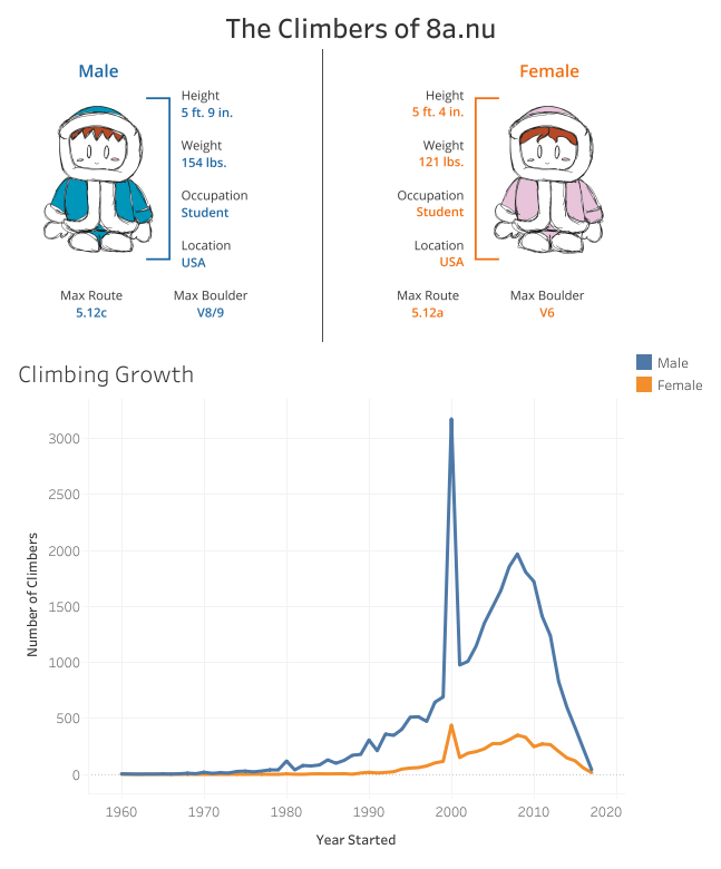
1. Climbing popularity starts climbing exponentially (pun intended) from around the year 1990 for men, and around the year 2000 for women.
1. The growth of female climbers is slower than male climbers, with a slight lag.
2. There is an unexplained peak in the year 2000 which may be an artifact of the database. Perhaps this is the default value given if left empty.
2. The vast majority of users on 8a.nu (86%) are male.
3. Females are, on average, 27 lbs lighter and 5 inches shorter than males.
4. Males tend to climb a few grades above females in both bouldering and route climbing (possibly due to user bias).
5. Most astonishingly, we can see that the average user on 8a.nu is quite strong! The average grade of a boulder climb was V6-V8/9, and the average grade of a route climb was 5.12a-c, both of which are considered an advance to expert level (https://www.guidedolomiti.com/en/rock-climbing-grades/)!

Conclusion

I hope you enjoyed our journey in trying to discover key insights about the climbing community through data analysis with SQL and Python. Please stay tuned for more as I am actively building an application that tries to predict the maximum bouldering grade you can climb given a user’s features!

Acknowledgements

Jane Choi helped formulate questions, find datasets, and created all the designs featured in the Tableau dashboard.